In this section we will discuss the status of the HET facility and each instrument and any limitation to configurations that occurred during the period.
NOTE: We are now using FWHM which is measured off both the LRS "pre" images and the FIF bent prime guider.
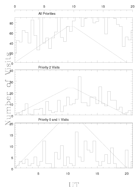
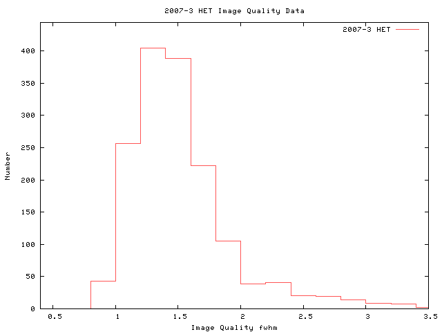
Here is a histogram from the last period.
For comparison here is the image quality for the period last year.
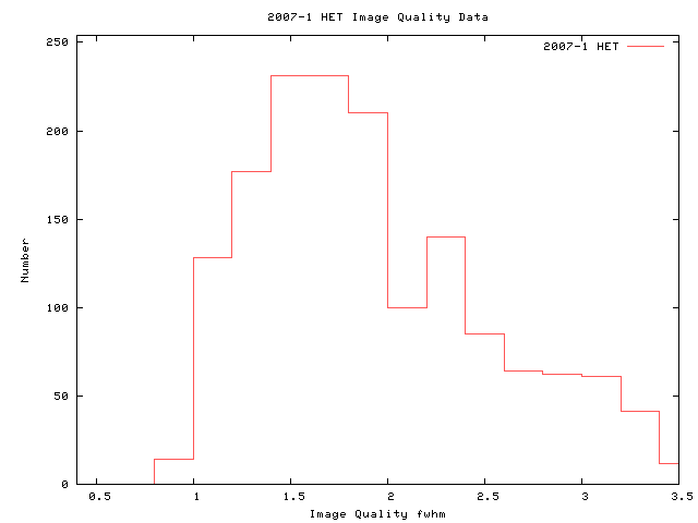
We expect to do about as good as the previous period and year. Note we have changed from a GFWHM on the LRS to a FWHM and we are measuring the FWHM on the ACQ camera using the same software.
We expect to have a similar overhead to last period. The following overhead statistics include slew, setup, readout and refocus between exposures (if there are multiple exposures per visit). In the summary page for each program the average setup time is calculated. The table below gives the average setup time for each instrument PER REQUESTED VISIT AND PER ACTUAL VISIT. The table also gives the average and maximum PROPOSED science exposures and visit lengths.
The "Exposure" is defined by when the CCD opens and closes. A "Visit" is the requested total CCD shutter open time during a track and might be made up of several "Exposures". "Visit" as defined here contains no overhead. To calculate one type of observing efficiency metric one might divide the "Visit" by the sum of "Visit" + "Overhead".
The average overhead per actual visit is the overhead for each acceptable priority 0-3 (not borderline, and with overheads > 4 minutes to avoid 2nd half of exposures with unrealistically low overheads) science target. This number reflects how quickly we can move from object to object on average for each instrument, however, this statistic tends to weight the overhead for programs with large number of targets such as planet search programs.
The average overhead per requested visit is the total charged overhead per requested priority 0-3 visit averaged per program. To get this value we average the average overhead for each program as presented in the program status web pages. The average overhead per visit can be inflated by extra overhead charged for PI mistakes (such as bad finding charts or no targets found at sky detection limits) or for incomplete visits e.g. 2 visits of 1800s are done instead of 1 visit with a CRsplit of 2. The average overhead per visit can be deflated by the 15 minute cap applied to the HRS and MRS. This method tends to weight the overhead to programs with few targets and bad requested visit lengths, ie. very close to the track length.
| Instrument | Avg Overhead per Actual Visit(min) | Avg Overhead per Requested Visit(min) | Avg Exposure (sec) | Median Exposure (sec) | Max Exposure (sec) | Avg Visit (sec) | Median Visit (sec) | Max Visit (sec) |
|---|---|---|---|---|---|---|---|---|
| LRS | 14.6(from last period) | 14.1(from last period) | 633.4 | 600 | 1800 | 1165.3 | 600 | 3600 |
| HRS | 8.2(from last period) | 9.1(from last period) | 699.1 | 708 | 1800 | 857.5 | 800 | 6600 |
| MRS | 9.6(from last period) | 9.8(from last period) | 762.2 | 720 | 2100 | 841.1 | 1080 | 2100 |
NOTE: AS OF 2003-3 THE SETUP TIME FOR AN ATTEMPTED MRS OR HRS TARGET IS CAPPED AT 15 MINUTES.
NOTE: STARTING IN 2004-3 THE SETUP TIME FOR AN ATTEMPTED LRS TARGET WILL CAPPED AT 20 MINUTES.
The overhead statistics can be shortened by multiple setups (each one counted as a separate visit) while on the same target as is the case for planet search programs. The overhead statistics can be lengthened by having multiple tracks that add up to a single htopx visit as can happen for very long tracks where each attempt might only yield a half visit.
A way to improve the overhead accumulated for programs with long exposure times is to add double the above overhead to the requested visit length and make sure that time is shorter than the actual track length. This avoids the RA having to split requested visits between several different tracks.
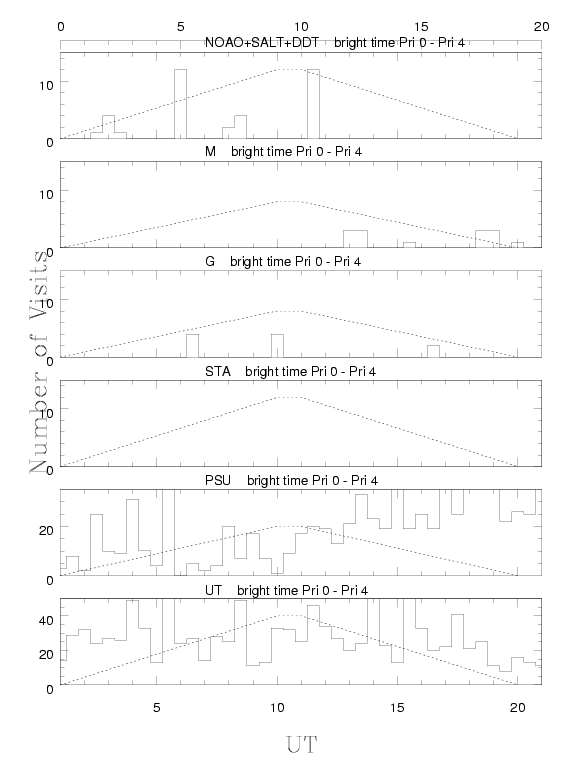
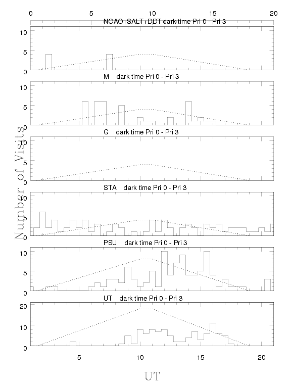
The following links give the summary for each institution and its programs.
The resulting table will give (for each program) the total number of targets
in the queue and the number completed, the CCD shutter open
hours, average overhead for that program, and the TAC allocated time.
This usually will be the best
metric for judging completeness but there are times when a PI will tell
us that a target is "done" before the total number of visits is complete.
This is how each institution has allocated its time by priority.
Observing Programs Status
Program comments:
UT08-1-001: (Wheeler) priority 1-2 LRS, TOO SDSS SN program run by STA07-3-001
UT08-1-003: (Cochran) priority 1-4 HRS
UT08-1-004: (Lambert) priority 4 MRS
UT08-1-005: (Barnes) priority 4 , HRS
UT08-1-006: (Benedict) priority 0-4 HRS
UT08-1-007: (Hill) priority 2 LRS
UT08-1-008: (Ramirez) priority 2-3 HRS
UT08-1-009: (Williams) priority 4 HRS
UT08-1-010: (Williams) priority 2-3 LRS
UT08-1-011: (Redfield) priority 1-2, HRS
UT08-1-012: (Redfield) priority 1-3, HRS
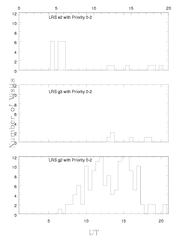
UT08-1-013: (Fisher) priority 1-2 LRS e2
UT08-1-014: (Sneden) priority 1-4 HRS
UT08-1-015: (Falcon) priority 2-3, HRS
UT08-1-016: (Robinson) priority 1-2 MRS
UT08-1-017: (Siegel) priority 1,3 HRS
UT08-1-018: (For) priority 3 HRS
UT08-1-019: (Wheeler) priority 0-2 LRS, TOO
UT08-1-022: (Kormendy) priority 1 LRS
UT08-1-023: (Cochran) priority 0-1 HRS
Program comments:
PSU08-1-001: (Wolszczan) priority 3-4 HRS
PSU08-1-002: (Wolszczan) priority 1-4 HRS
PSU08-1-003: (Miller) priority 2-3, LRS g2
PSU08-1-004: (Miller) priority 2, LRS g2
PSU08-1-005: (Miller) priority 3, LRS
PSU08-1-006: (Gronwall) priority 2, LRS g2
PSU08-1-007: (Chartas) priority 0, LRS g3,
PSU08-1-008: (Fox) priority 0-1, LRS, TOO
PSU08-1-009: (Fox) priority 2-4 LRS g2,
PSU08-1-010: (Schneider) priority 1, LRS, TOO SDSS SN program run by STA07-3-001
PSU08-1-012: (Eracleous) priority 1-4, LRS g3
PSU08-1-013: (Eracleous) priority 3-4, LRS g2
PSU08-1-015: (Brown) priority 0, LRS, TOO
PSU08-1-016: (Gibson) priority 2-3, LRS g2
PSU08-1-018: (Gibson) priority 2, LRS g2
PSU08-1-019: (Wade) priority 1-2, HRS
PSU08-1-020: (Wade) priority 0-2, HRS
PSU08-1-021: (Brandt) priority 1-2, LRS g2
PSU08-1-022: (Brandt) priority 2, NO PHASE II
PSU08-1-101: (Wolszczan) priority 0-1, HRS
Program comments:
STA08-1-001: (Romani/Sako) priority 0-3 LRS g1, SN program
STA08-1-002: (Romani/Michelson) priority 1-4 LRS g1
Program comments:
M08-1-001: (Saglia) priority 1-2, LRS e2
M08-1-002: (Saglia) priority 2-3, NO PHASE II
M08-1-003: (Saglia) priority 0, LRS E2
M08-1-004: (Hopp) priority 0,2, SN program run by STA07-3-001
M08-1-005: (Hopp) priority 1-3, LRS g2
M08-1-006: (Goessl) priority 0,2-3, LRS g2
M08-1-007: (Burwitz) priority 2-3, LRS
M08-1-008: (Seitz) priority 1-2, LRS NO PHASE II
M08-1-009: (Bender) priority 0,2-3, LRS E2
M08-1-010: (Riffeser) priority 0-1, LRS g1 TOO
Program comments:
G08-1-001: (Kollatschny) priority 1-3 LRS g2
G08-1-002: (Schuh) priority 2 HRS
G08-1-003: (Bean) priority 2 HRS
Institution Status
| Time Allocation by Institution (hours) | |||||
|---|---|---|---|---|---|
| Institution | Priority 0 | Priority 1 | Priority 2 | Priority 3 | Priority 4 |
| PSU | 11.170 | 30.100 | 36.670 | 36.670 | 64.570 |
| UT | 19.000 | 69.350 | 86.000 | 87.000 | 79.000 |
| Stanford | 4.000 | 8.000 | 12.0000 | 12.000 | 6.000 |
| Munich | 8.000 | 8.000 | 17.000 | 14.000 | 0.000 |
| Goetting | 0.000 | 3.500 | 13.5 | 3.500 | 0.000 |
| NOAO | 0.000 | 30.560 | 71.160 | 16.000 | 0.000 |
| SALT | 0.000 | 0.000 | 0.000 | 0.000 | 0.000 |
| DDT | 0.000 | 0.000 | 0.000 | 0.000 | 0.000 |
Stanford and Goetting have under allocated time to their institutional share. Munich put in sufficient hours for this period but we could use more Munich targets to assist in their total deficit.